An important characteristic of the Midpoint Rule is that the approximation tends to improve as n increases.
The next Table shows the approximations for the area of the region described in the Example in the previous web page.

n 5 10 15 20 25 30
Approxi-
mation
7.36 7.34 7.3363 7.3350 7.3344 7.3341

For example, for n = 10, the Midpoint Rule yields the following approximation.

0 2 ( - x 2 + 5 ) d x 2 10 [ f ( 1 10 ) + f ( 3 10 ) + f ( 5 10 ) + f ( 19 10 ) ] =
7.3400

Note from this table that as n increases the approximation appears to be getting closer and closer to the exact value of the integral, which we found to be
22 3 7.3333

In fact, taking the limit as n approaches infinity makes the approximation exact. That is, if x = b - a n  , then

a b f ( x ) d x = lim n &to; &infty; [ f ( x 1 ) Δ x + f ( x 2 ) Δ x + &cdots; + f ( x n ) Δ x ]

For the Midpoint Rule we choose x i to be the midpoint of the i-th subinterval.
However, in the limit form, x i can be any number in the i-th interval, as shown in the next figure.

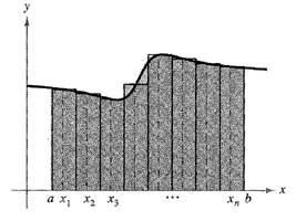
n subintervals, each of width x = b - a n

We summarize this result as follows.

Definite Integral as the Limit of a Sum
If a function  f is continuous on the closed interval  [a,b] then
a b f ( x ) d x = lim n &to; &infty; [ f ( x 1 ) Δ x + f ( x 2 ) Δ x + &cdots; + f ( x n ) Δ x ]
where   x = b - a n   and   x i   is any number in the ith interval.

In the the Example from the previous web page, we used the Midpoint Rule to approximate the area of the region bounded by the graph of f ( x ) = - x 2 + 5   and the x-axis between  x = 0 and  x = 2. Of course, for this particular region we wouldn't normally go to the trouble of approximating the area, since we can find the exact area by evaluating the definite integral

0 2 ( - x 2 + 5 ) d x

The real usefulness of the Midpoint Rule lies in its application in the problems where we encounter definite integrals that we don't know to evaluate. This demonstrated the examples.