STROJNÉ INŽINIERSTVO 2000   15. NOVEMBER 2000 STROJNÍCKA FAKULTA STU BRATISLAVA

Projections and their Classification

Dagmar Szarková* - Kamil Maleček**

  *Department of Mathematics, Faculty of Mechanical Engineering,

Slovak University of Technology

E-mail: szarkova@sjf.stuba.sk

** Department of Mathematics, Civil Engineering Faculty,

Czech Technical University

E-mail: kamil@mat.fsv.cvut.cz

Abstract

In this paper a general geometric definition of a projection is introduced. We will work in detail with the projection, where the plane stands for the image surface and lines forming the congruence of lines in 3-D space are projecting curves. The basic distribution to linear and quadratic projections is introduced with their further classification. In this paper analytic representations of projections suitable for computer processing are derived. Views of a single machine part in different types of projections produced by means of computer are shown.

  I.     Generally about projection

Let r be a two-dimensional surface in the extended Euclidean space E³.

Any mapping P of the space E³ onto the surface r is called a projection. The surface r is called an image surface. The point X’ is the image of the point X, if  X’ = P(X),  X’Îr .

In geometry we introduce the projection P in this way:

Let us define the system S of curves, while any s, s Î S will by denoted as a projecting curve. The system S has the following properties:

i)      One and only one curve s^X,  s^XÎS is passing through almost any point XÎE³, s^X is the projecting curve of the point  X .

ii)  Any projecting curve has one and only one common point with the image surface.

The point  X’ is an image of the point  X  in a projection, when the point  X’ is an intersection point of the projecting curve s of the point  X with the image surface r.

The domain of definition of the projection P is the set of all points X, which have the image in the projection.

The projection is determined by the image surface r and by the system of projecting curves. The choice of the image surface r and system of projecting curves gives different types of projections. The most frequently used projection is the one, where the image surface r is a real plane and projecting curves are lines. The reasons are obvious. Any line s, s Ër, has one and only one point in common with the plane r in the space E³. We will use this projection only, in the following.

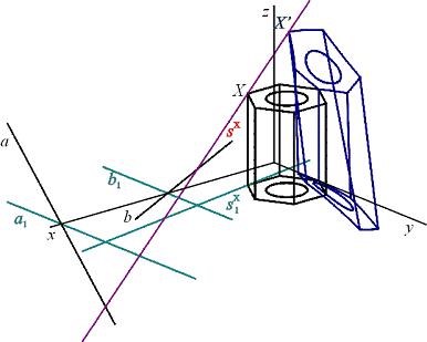
II. Projection  P(r, a, b)

In the Euclidean space E³, let us choose two different lines a, b  that are not located in the image plane r. Let the projecting line be any line intersecting lines a and b. This projection will be marked  P(r, a, b).

According to mutual position of lines a, b we get the following types of projections
P(r, a, b):

1. Linear projection

The lines a, b have one and only one common point  S, S  r and therefore they determine the plane w. The domain of definition is D(P) = E³ – {w}.

a)  If the point S = a Ç b is a finite point, then a projecting line of any point X  w is the line  SX. Let the projecting lines of the points XÎw,  X  S  are also lines SX . Then we speak about central projection with the centre  S . The domain of definition is D(P) = E³ – {S}.

b)      If the point S = a Ç b is a point at infinity, then the projecting line  s^X of any point  X w   is the line  SX . Let the projecting lines of points  XÎw,  X  S are also lines SX . Then we speak about parallel projection with the direction s = s^X. The domain of definition is

      D(P) = E³ – {S}.

2.  Quadratic projection

The lines a, b are two skew lines. The projecting line of the point X  (X  a   X  b) is the line passing through the point X and intersecting both skew lines a, b .

The domain of definition is D(P) = E³ – {a b }. This projection is called quadratic projection. The image in the quadratic projection will be denoted as quadratic view.

The quadratic projections can be also classified similarly as the linear projections mentioned above:

a)  both lines a, b are real lines,

b)  the line a is the real line and the line b is the line at infinity, the latter being determined by the real plane b not parallel to the plane r and intersecting the line a .

J. Klíma studied the quadratic projection [1] , which is closely connected to the congruencies of lines. He named it the net projection. The notion quadratic projection is probably more proper because generally the image of a line is a conic section. It is therefore evident that a computer can more precisely construct the quadratic view of any object.

III.  Analytic representation of quadratic projection in the space E³

In the Euclidean space E³ let us choose a Cartesian coordinate system O, x, y, z so that the projection plane r be the plane yz. Let the point X ΠD(P) have the coordinates [x, y, z] and the point X’ with coordinates [x´, y´, z´] be its image.

a)     Let the line a be determined by the point A = [x_A, 0, 0] and by the direction vector a = (x_a, y_a, z_a) . The line b will be determined by the point B = [x_B, 0, 0] and by the direction vector b = (x_b, y_b, z_b) .

The projection defined in this way has the analytic representation

b)    Let the line a be determined by the point A = [x_A, 0, 0] and by the direction vector

a = (x_a, y_a, z_a) . The line b will be line at infinity determined by the direction vector

b = (x_b, y_b, z_b) and by the point B, which is the point at infinity determined by the vector (x_B, y_B, z_B) .

Analytic representation of this projection is

Now we will introduce two particular examples of a quadratic projection and we will present quadratic views of a simple machine part under these projections. 

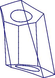
Example 1:

The line a is determined by the point A = [20, 0, 0] and by the direction vector a = (0, -1, 1).

The line b is determined by the point B = [10, 0, 0] and by the direction vector b = (0, 1, 1).

We obtain from equations (1) the analytic expressions

The quadratic view of the machine part under this quadratic projection is shown in Figs.1a and 1b.

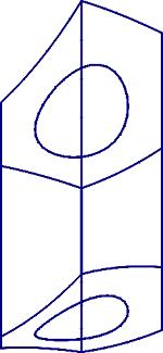
Example 2:

The line a is determined by the point A = [20, 0, 0] and by the direction vector a = (0, -1, 1)  (see example 1). The line b is the line at infinity and it is determined by the plane xy . We obtain the analytic representation (4) of this projection from the equations (1)

 In Figs. 2a and 2b there is the quadratic view of the machine part.

References

[1]  Klíma,J.: Různé způsoby zobrazovací v DG, Cesta k vědění sv.27, 1944.